HRUweb Tutorial
The HRUweb is a web tool which was developed to delineate hydrological response units (HRU) online. It was implemented in Python and calculates HRUs according to open-source GRASS-GIS algorithms.
After every processing step, the results are provided as raster or shape data which are all compatible with established GIS formats.
For this tutorial, sample data from Rio de Janeiro in Brazil were used.
Starting HRUweb Tool
Link to HRU Tool: http://intecral.uni-jena.de/hruweb-qs
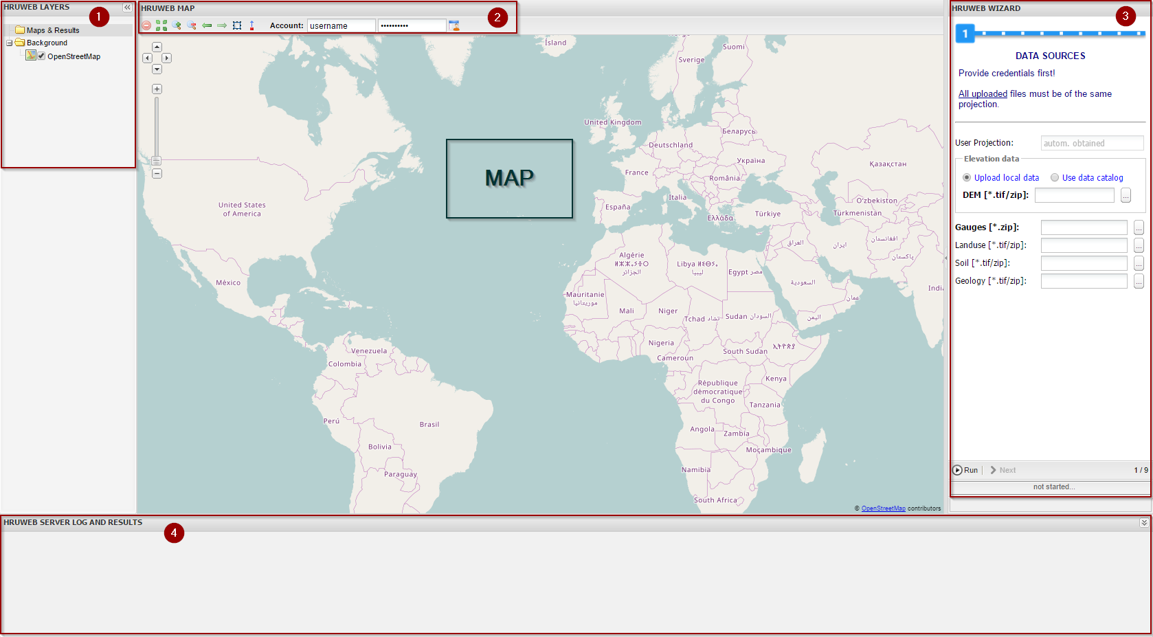
Structure of HRUweb user interface
The map window is located in the centre. By using the arrow buttons or the +/- tool bar in the top left, the view can be set manually. The remaining items are located around the map:
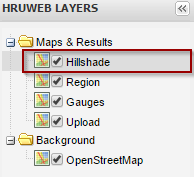
- Table of Layers
- Change order of layer visibility by using drag and drop
- Select a layer by clicking on it. Now the layer can be edited by using the Map Legend.
- Map Legend (→ section Map Legend Description see below)
- Wizard: Processing step description and manual input/settings. Includes the buttons for ‘Run’ and ‘Next’.
- Server Log and Results: Shows the uploading process & provides the result layer as raster or shape file. (→ click on
 to reveal the item and to hide it again)
Map Legend Description

- Remove layer
- Zoom to map extend: restores smallest possible scale of the map
- Zoom in the map (
 ) or zoom out of the map (
 )
) - Zoom to previous map extend (backward
 forward)
 - Create bounding box of interest (→ section Step 2)
- Relocate gauge (→ section Step 6)
- User login (→ NEXT STEP)
Step 0: Check Your Data
First of all: Do user login!
Otherwise, your work will not be saved!

Check your input data!
Then, open your input data in a GIS and check them for:
- completeness: At least DEM and gauges are required for delineating HRUs. The rasters of landuse, soil and geology are optional input.
- projection: The coordinate system has to be metric (like e.g. UTM) in order to enable distance calculations.
- layer extend: The layers should have at least the size of the catchment. A base map could be helpful.
| Input data | Description | Format | |
|---|---|---|---|
| DEM | Raster of Digital Elevation Model | Tiff (.tif) or .zip-file | mandatory |
| Gauges | Layer of gauging stations | .zip-file | mandatory |
| Landuse | Raster of landuse | Tiff (.tif) or .zip-file | optional |
| Soil | Raster of soil | Tiff (.tif) or .zip-file | optional |
| Geology | Raster of geology | Tiff (.tif) or .zip-file | optional |
All datasets that are uploaded as ZIP archives need to comply to the following rules:
- The archive must not contain any subdirectories
- The archive’s name (before .zip) must be identical to the file name(s) inside (e.g., if your Shapefile consists of multiple files named outlets.shp, outlets.dbf, outlets.prj etc., your ZIP archive must be named outlets.zip).
The following sections describe the single substeps in the HRUweb Tool. Each substep is divided into the subsections Aim, Procedure and Results.
Step 1: Define Data Sources
Aim: Upload input data or choose data via catalog.
Procedure:
The required input data are described in Step 0.
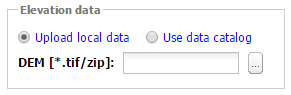
You have two options to define the dem input data:
-
Upload your own local input data
or
-
Use input data via catalog: choose the DEM you need by clicking on ‘add’.
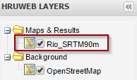
- Note: The chosen DEM is listed in the Table of Layers as a new layer. You can edit it by clicking on the layer and using the Map Legend.
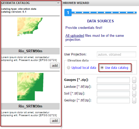
The projection of the map will be set automatically on the basis of the input data.
For starting the uploading process, click ‘Run’ in the Wizard.

Results:
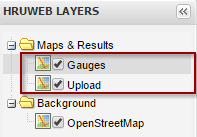
The overlays ‘Upload’ and ‘Gauges’ are created in the Map View as well as the Table of Layers.
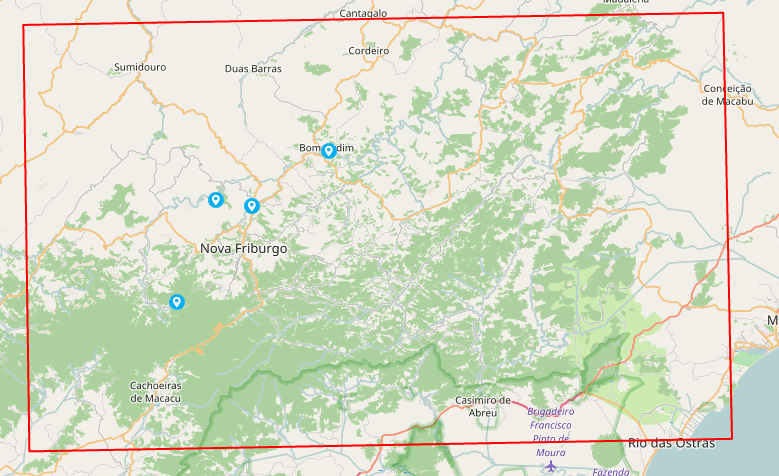
Zoom into your area of interest. The gauges are shown in light blue dots. The area of the gauges is marked automatically in a red bounding box.
Note: If the ‘Upload’ or the ‘Gauges’ layer are removed, the whole uploading procedure has to be done again by reloading the page.
When finished, click ‘Next’.
Step 2: Data Setup
Aim: Define area of interest for delineating HRUs.
Procedure:
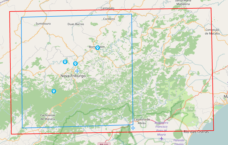
In this step, you can specify your region of interest. The red box marks the maximum extend. Data outside of this extend are not delineated.
Note: If the red bounding box does already represent your region of interest, you can skip the next step and click ‘Run’.
If you want to specify your region of interest, click on the box symbol  in the Map Legend.
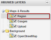
By clicking on the symbol, another overlay layer called ‘Region’ is created.
The automatically set red bounding box is now covered by a blue box.
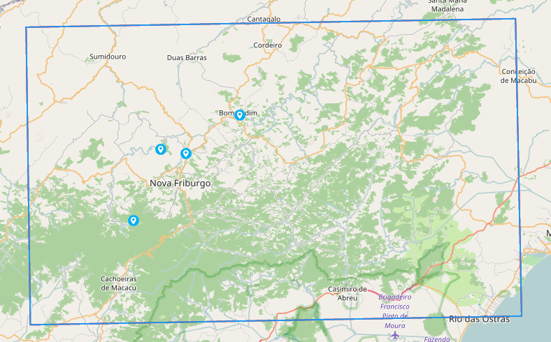
This blue box represents the area that should be used for delineating HRUs later on. Due to computational reasons, its extend should be fitted to the gauges’ positions.
Fit it by clicking on the outline of the blue box and move it at the blue crosses  .
.
In order to shift the whole box, drag & drop it by the blue cross in the centre. In order to resize the box, use the cross at the side.
Note: The ‘Region’ layer can be removed without problems. To do so, right-click on the layer and choose “remove”. By clicking on , the region layer can be restored again.
Note: If the extend of the blue box is chosen too small, important parts for delineating HRUs could be left out which makes the results unusable.
For starting the process, click ‘Run’.
Results:
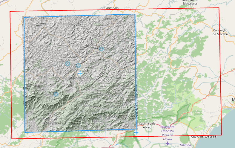
A ‘Hillshade’ overlay is created in the Table of Layers and showed in the Map.
When finished, click ‘Next’.
Step 3: Data Preparation
Aim: Preprocess the DEM by filling its sinks.
If the DEM was already preprocessed that way, no sink filling is necessary.
Otherwise, it is recommended to do so in order to prevent lack of data.
Procedure:
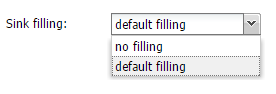
Choose “Filling” (default) in the Wizard window, if the sinks should be filled or “No filling”, if they should not be filled.
For starting the process, click ‘Run’.
Results:
A DEM with filled sinks is created. Single maps of sinkless elevation, slope and aspect can be downloaded from Server Log.

Note: If filling fails, no maps for slope and aspect are available.
When finished, click ‘Next’.
Step 4: Reclassification
Aim: Reclassify terrain attributes.
Procedure:
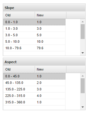
In this step, the class ranges of slope and aspect can be reclassified and renamed.
In order to change table entries, click in the concerning field and type in the desired value.
“Old”: lists all existing class ranges
“New”: assigns IDs to classes
HELP
How to choose the best settings for ranges of values of slope and aspect?
For starting the process, click ‘Run’.
Result:
The reclassified layers ‘aspect’ and ‘slope’ are listed in The Table of Layers.
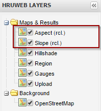
Aspect and slope are also shown as maps.
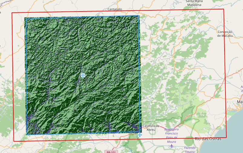
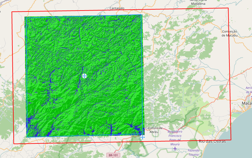
The reclassified maps of slope and aspect can be downloaded from Server Log as well.

When finished, click ‘Next’.
Step 5: Waterflow
Aim: Define resolution of the stream network/river system.
Procedure:
With each subbasin, one river segment is created. In this step, the maximum number of cells (pixels) for a subbasin of the smallest size has to be specified.

In this tutorial, the cellsize was defined by 10.000 pixels.
HELP: HOW TO FIND THE BEST MAXIMUM CELL SIZE FOR THE SMALLEST SUBBASIN? / choose the best settings for number of pixels for the smallest subbasin
Depending on, how detailed the river network does look like. Compare to Google Earth.
For starting the process, click ‘Run’.
Results:
The layers ‘Streams’ and ‘Subbasins’ are created.
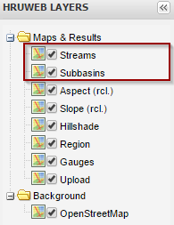
In the map view, the subbasin as well as the stream network layer are shown.
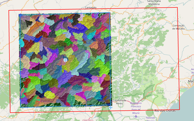
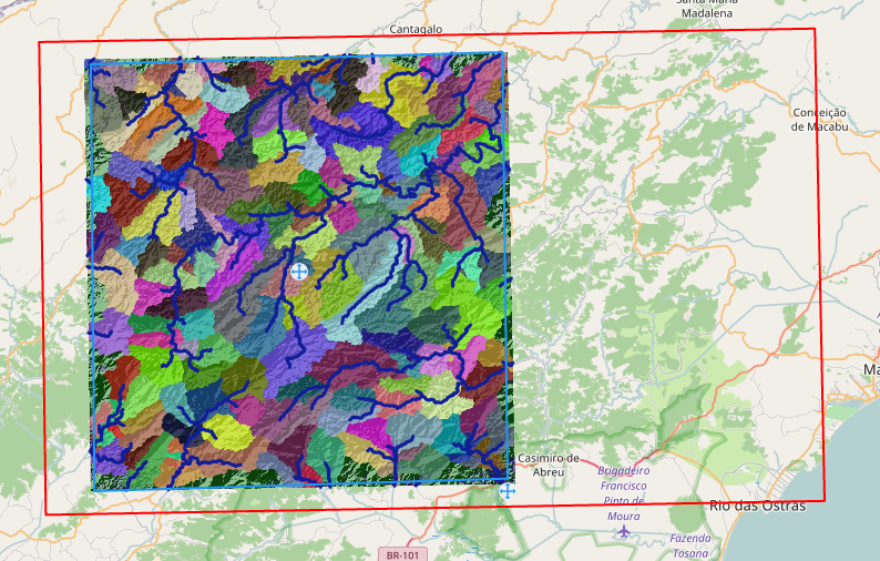
You can download a map of the subbasins in raster and shape format and a vector zip file of stream network from Server Log.

When finished, click ‘Next’.
Step 6: Outlets
Aim: Check the gauges’ position and decide which gauges should be considered.
While creating the subbasins, the gauges’ position can differ from the stream network.
Procedure:
First of all, use the drag and drop mechanism to change the visibility of the layers in the layer view (→ section Starting the Webtool). Order the layer of gauges on top, followed by the layer of streams and the subbasins.
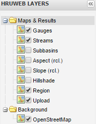
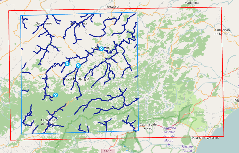
→ Check gauges:
- Context: Take a look on the hydrological data - What kind of river properties (amount/velocity of discharge, water level, etc.) were measured? Are the data comprehensible compared to their position in the map?
- Google Earth: You can save your shapefile of gauges as a .kml-file and open it in Google Earth. Then zoom in to the gauges. The satellite imagery can be a helpful reference to verify the position of the gauges.
Note: The positions can differ significantly in Google Earth, so always doublecheck the positions by its hydrological context!
Now the tool for relocating gauges had to be activated. Click on  in the legend to activate it. In order to relocate a gauge, click on a gauge and drag it to the proper river segment.
Note: For every gauge on a river segment, a catchment is created. If a gauge should not be considered in the further delineation of HRUs, just drag it out of the blue bounding box.
When you are finished, click on to deactivate the tool again!
For starting the process, click ‘Run’.
Note: If you forgot to deactivate the tool, wait until the process is finished and deactivate the tool. Now click on ‘Run’ again.
Results:
The layer ‘Watershed’ is listed in the Table of Layers.
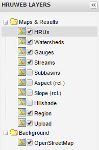
A map of the watersheds is shown in the Map View and can be downloaded from Server Log.
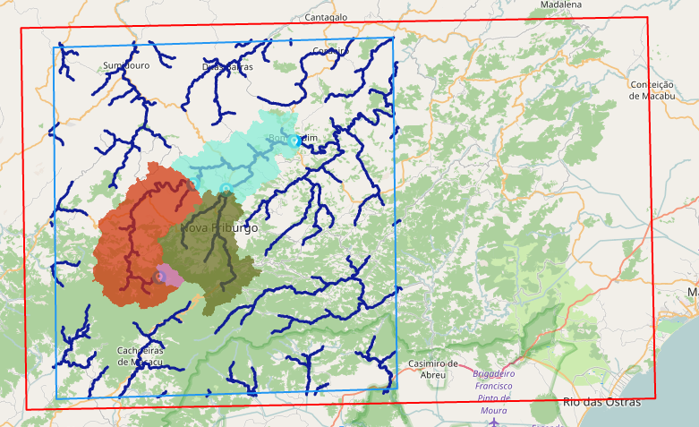

When finished, click ‘Next’.
Step 7: Dataoverlay
Aim: Computing HRUs.
Procedure:
Specify the number of cells (pixels) for the smallest HRU in the wizard. In this tutorial, the number of the smallest HRU was defined by 10.

HELP: HOW TO FIND THE BEST NUMBER OF CELLS FOR THE SMALLEST HRU?
- HRU should cover between 1-10 ha (10.000 - 100.000 m²) → depends on cell size of the dem used.
For starting the process, click ‘Run’.
Results:
The layer ‘HRU’ is created in the layer overview and shown in the map view.
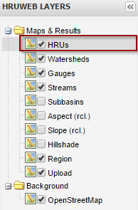
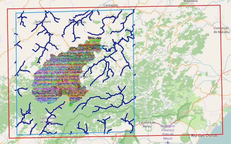
A map of the created HRUs is provided in the server log.

When finished, click ‘Next’.
Step 8: Routing
Aim: Creating topology information.
Procedure:
In this step, all calculations are done by the WebTool. No user activity is required here.
For starting the process, click ‘Run’.
Results:
All routing parameters are available in the server log. They are provided as .csv-tables.

When finished, click ‘Next’.
Step 9: Statistics
Aim: Collecting statistics per HRU.
Procedure:
In this step, all calculations are done by the WebTool. No user activity is required here.
For starting the process, click ‘Run’.
In order to see the results, click ‘Next’.
Results:
Shapefiles of the HRUs as well as their parameters can be downloaded from the server log.

The results of all steps can be downloaded in a zip-file.

FINISHED
If the delineation shall be repeated, click on:
