Efficiency Calculation
Overview
Model efficiency calculation is essential for assessing model quality and guiding automated calibration. Access this feature via Model -> Configure Efficiencies in the JAMS builder.
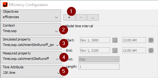
Basic Setup Steps
- Select an objective or create a new one (1). In the second case, please provide a name.
- Select your main time iteration context (2)
- Select the attribute representing your simulated property (3)
- Select the attribute representing your observed property (4)
- Select the time attribute (5)
- Press OK
A new component will be inserted at the end of your selected time iteration context with the same name as your chosen objective (see for example Figure 2).
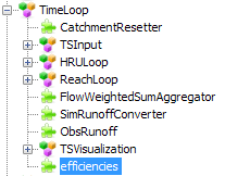
Efficiency Metrics Calculated
The newly added component calculates several efficiency criteria at simulation end:
- R2: Coefficient of determination
- (log) E1/E2: (Logarithmic) Nash-Sutcliffe-Efficiency
- AVE: Absolute volume error
- Bias: Percental bias
- KGE: Kling-Gupta Efficiency
All efficiency measures except AVE and Bias are also calculated in a normalized form, where 0 denotes their optimal value.
Time Filters Configuration
By default, the full simulation period is used. However, you can limit efficiency calculation to specific sub-intervals or events.
Steps to Add Time Filters
- Open the efficiency configuration dialog
- Select your efficiency set from the Objectives pull-down list
- Press the Load Timeserie button (1) and choose a measured runoff timeserie, or select an entry from the list next to it (2). The chosen timeserie will be shown in a graph (3).
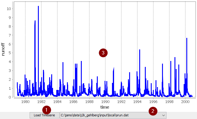
- Press “+” in the Time Filters table to add a new filter
- Configure filter options:
- Select one or more years
- Select one or more months
- Select baseflow situations (threshold or local minimum)
-
Select raising/falling limbs or peaks of the timeserie based on a time window size and the distinctness of the situation:
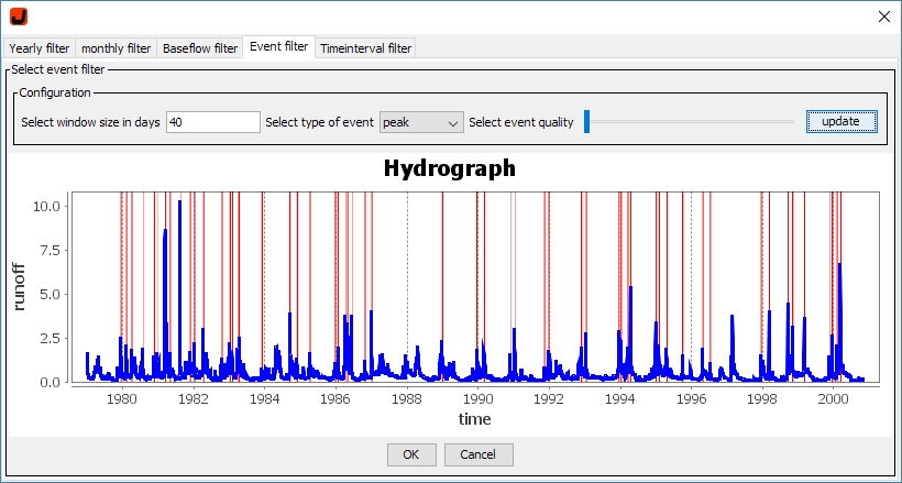
- Select arbitrary time intervals
- Confirm with OK in order to add the selected time intervals (shown in red) to the Time Filters table
- Repeat steps 4/5 to add more filters. Each of the filters is shown in the filter table and can be enabled/disabled
Filter Configuration Options
After different filters have been created, users can further configure them in the Time Filters table, i.e. by defining
- how they are combined (logical AND/OR)
- if they should be inverted
- if they should be enabled or disabled
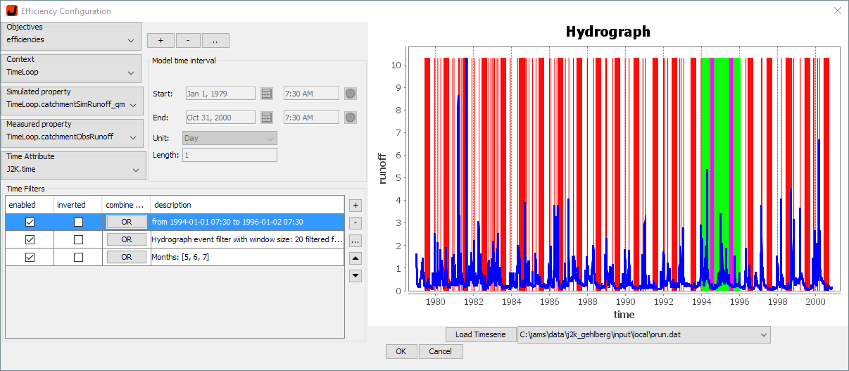
An overview of the resulting filter setup is shown in a graph on the right hand side of the window. Figure 3 shows an example of three filters that are combined by logical OR:
- time interval 1994-1996 (enabled and highlighted in green)
- peak events
- months May to July
Application
Using these efficiencies in a following parameter calibration allows you to focus on specific requirements of the simulation, such as flood event identification or minimal flow assessment.