Spatio-temporal Data Aggregation
Spatially distributed environmental models generate a lot of spatio-temporal data. To work with these data effectively it is usually necessary to aggregate it and to visualize it in maps. This article shows how JAMS can be used to aggregate spatio-temporal data and to save the result in a shapefile. To demonstrate the workflow, a map of yearly mean precipitation is generated for the Wilde Gera catchment at gauge Gehlberg with the model J2000. This model is shipped with every JAMS installation (j2k_gehlberg.jam).
Preparing and running the model
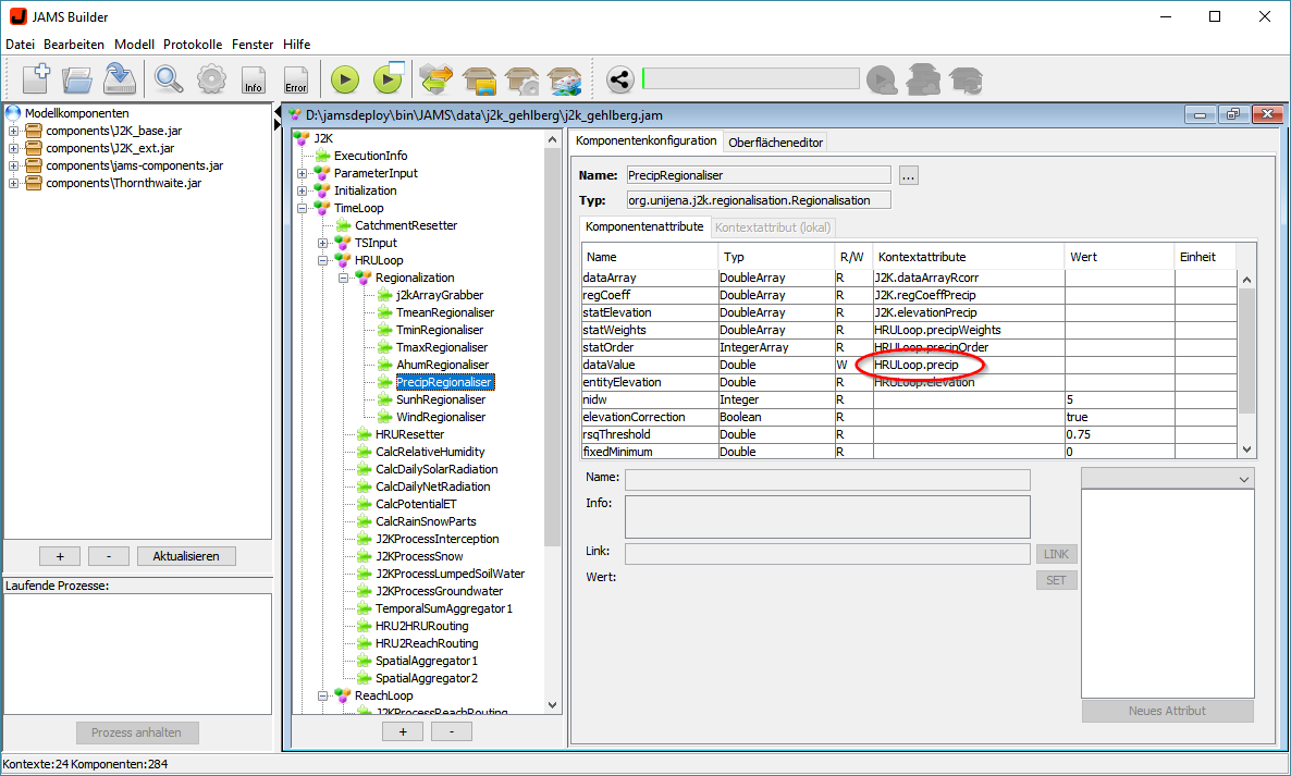
Start by opening the model in the JAMS User Interface Configuration Editor (JUICE) and have a short look at the model structure. The model has a J2K model context, which contains the temporal context named TimeLoop. A spatial context named HRULoop is nested within TimeLoop. The precipitation values are stored in the attribute precip within the HRULoop context.
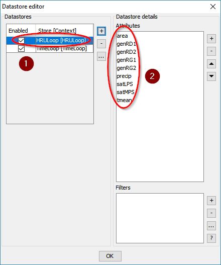
Now ensure that the spatially distributed precipitation data, calculated by J2000, is actually saved in a file. For that purpose, use the Configure Model Output  function from the toolbar. The datastore editor dialog will show up, which allows you to configure the model outputs. On the left side of the dialog you see a list of all output datastores already configured. By means of the +, − and … buttons you can easily add, edit or rename a datastore. By selecting a datastore in the list, its chosen output attributes are shown in the list on the right side of the dialog. To enable outputs for the spatial context, tick HRULoop on the left side. With the plus and minus buttons on the right you may add the precip and area attribute to the list and delete all other attributes. Please note that both outputs are already preconfigured in the Wilde Gera example model.
Now start the model. During the model run, JAMS will output the chosen attributes of the HRULoop datastore at each time step and for each spatial model unit. The execution will take a moment (23 seconds on the reference machine), because saving the large amount of data requires some additional time. The results are saved in a file named HRULoop.dat which is located in the output directory.
Using JAMS Data Explorer (JADE)
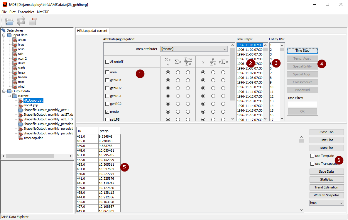
After the model finished its simulation, open the JAMS Data Explorer (JADE) from the toolbar  or by pressing CTRL+J. When JADE shows up, you should see HRULoop.dat on the left side already. Double-click on HRULoop.dat to open it. Now you should see a data view as shown in figure 3. Region 1 shows all attributes within the selected file. In our case it contains the preconfigured attributes, namely area, genRD1/2, genRG1/2, precip, satLPS, satMPS, and tmean. Region 2 shows, for which time steps data is available. J2000 is a daily model and in this case the simulation was done from 1996-11-01 to 2000-10-31, so the list contains 1461 entries, one for each day. Region 3 lists the IDs for all spatial model units. For the Wilde Gera catchment, 614 entities (HRUs) are used. In region 4, several functions are available to process the data. Selecting one or more attributes (e.g. precip) and a time step, followed by pressing the Time Step button, extracts all data for that specific time step without further aggregation, generating a table in region 5. The first column of the table shows the IDs of all entities, the second column the precipitation value for each entity. Accordingly, selecting a single entity ID and pressing the Spatial Entity button shows a table with a time series of e.g. precip for that specific unit (HRU). Region 6 offers various functions to plot, analyze and export aggregated data.
Temporal Aggregation
Usually, it is not sufficient to inspect a single timestep. Instead you may want to aggregate the data. This can be done by selecting a number of time steps followed by using one of the aggregation functions. Selection of time steps can be done manually or automatically using wildcards:
Manual selection
- hold CTRL and select/unselect individual time steps
- click a first time step, hold SHIFT and click a second time step to select all in between
- click into the list and press CTRL+A to select all
Automatic selection
- type a search term into the Time Filter text box, using wildcards to match one or more time steps, e.g.
1997*to match all values in 1997*-10-*to match all October values*-*-01*to match all first days in all months
- press ENTER/OK to mark all matching time steps
After selection of time steps, you have to choose how data should be aggregated in time. This is controlled by two groups with three columns of radio buttons each (see figure 4). The first group (1) controls the type of aggregation:
 average: This will calculate the average of the values for the selected time steps
 sum: This will calculate the sum of the values for the selected time steps
 weighted average: This will calculate the weighted average of the values for the selected time steps. For this purpose, the area attribute (3) must have been selected before.
As far as time steps are usually equally long, there should be no need to use the weighted average option. However, depending on the unit of the aggregated attribute, a unit conversion may be required. This is handled by the options in the second group (2):
 leave the aggregated value untouched
 Divide the aggregated value by the average/overall area. For this purpose, the area attribute (3) must have been selected before.
 Multiply the aggregated value with the average/overall area. For this purpose, the area attribute (3) must have been selected before.
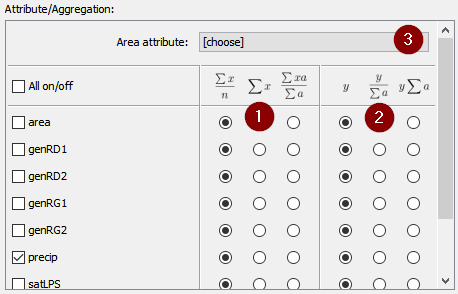
After selection of time steps, attributes and aggregation/conversion options, press the Temp. Aggr. button (figure 3, region 4) to start the data extraction process.
Examples
Calculate the average daily precipitation in liters:
- select all time steps (click into time step list and press CTRL+A)
- tick precip
- in the precip row, select the first radio button of group 1
- select the attribute area as the area attribute (3)
- in the precip row, select the third radio button of group 2 (since precipitation is stored in mm)
- press Temp. Aggr.
Calculate the overall surface runoff (genRD1) for 1998 in mm:
- enter
1998-*into the time filter field and press ENTER - tick genRD1
- in the genRD1 row, select the second radio button of group 1
- select the attribute area as the area attribute (3)
- in the genRD1 row, select the second radio button of group 2 (since genRD1 is stored in liters)
- press Temp. Aggr.
Exporting Data
At last, the aggregated data can be exported to other software. You may simply drag and drop the data to e.g. Microsoft Excel. Alternatively you can export the data to a text file or to a Shapefile. To save the data in a text file, use the Save Data button (figure 3, region 6). A dialog will show up, allowing you to select the location and name of the output file.
To save the data in a Shapefile, use the Write to Shapefile button. To use this function, you need a suitable Shapefile datastore in your input directory (see Spatio-temporal Data Visualization for how to configure one). If you have more than one Shapefile datastore in your input directory, you can select the right datastore in the combobox below the buttons.
Before saving the extracted data, select the desired columns by marking at least one cell of each column to be stored in the Shapefile (hold CTRL to mark multiple columns). Afterwards, press the Write to Shapefile button to continue. A dialog window will pop up asking where to save the new Shapefile. Once the location is confirmed, the data export will start, with progress messages shown along the way:

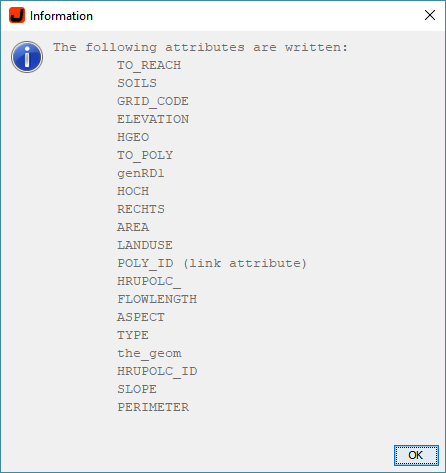
…and a final success message once the fields attached to the shapefile are confirmed.

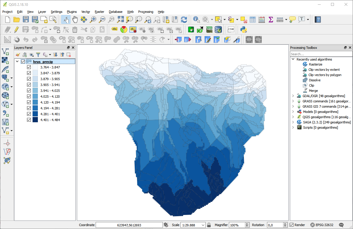
After that you can work with the newly created shapefile in a GIS software of your choice.